This page was generated from doc/examples/MatchHistory - Home advantage.ipynb.
You can download the notebook,

import soccerdata as sd

%matplotlib inline
%config InlineBackend.figure_format = 'retina'

import pandas as pd
import seaborn as sns

sns.set_context("notebook")
sns.set_style("whitegrid")

Home team advantage in the Italian Serie A

We all know sports teams have an advantage when playing at home. Here’s a look at home team advantage for 5 years of the Serie A.

seriea_hist = sd.MatchHistory("ITA-Serie A", range(2018, 2023))
games = seriea_hist.read_games()
games.sample(5)

			date	home_team	away_team	FTHG	FTAG	FTR	HTHG	HTAG	HTR	HS	...	AvgC<2.5	AHCh	B365CAHH	B365CAHA	PCAHH	PCAHA	MaxCAHH	MaxCAHA	AvgCAHH	AvgCAHA
league	season	game
ITA-Serie A	2223	2023-05-20 Cremonese-Bologna	2023-05-20 14:00:00	Cremonese	Bologna	1	5	A	0	3	A	13	...	1.8	0.50	1.84	2.06	1.85	2.08	1.90	2.15	1.83	2.03
	2021	2020-12-06 Crotone-Napoli	2020-12-06 17:00:00	Crotone	Napoli	0	4	A	0	1	A	4	...	2.3	1.25	1.99	1.94	1.98	1.94	2.03	1.96	1.96	1.90
	1819	2019-05-26 Fiorentina-Genoa	2019-05-26 12:00:00	Fiorentina	Genoa	0	0	D	0	0	D	5	...	NaN	NaN	NaN	NaN	NaN	NaN	NaN	NaN	NaN	NaN
	2021	2020-11-01 Udinese-Milan	2020-11-01 11:30:00	Udinese	Milan	1	2	A	0	1	A	7	...	2.0	0.50	1.95	1.98	1.93	1.99	1.99	2.01	1.93	1.94
	1819	2019-03-10 Frosinone-Torino	2019-03-10 12:00:00	Frosinone	Torino	1	2	A	1	0	H	9	...	NaN	NaN	NaN	NaN	NaN	NaN	NaN	NaN	NaN	NaN

5 rows × 121 columns

def home_away_results(games: pd.DataFrame):
    """Returns aggregated home/away results per team"""
    res = pd.melt(
        games.reset_index(),
        id_vars=["date", "FTR"],
        value_name="team",
        var_name="is_home",
        value_vars=["home_team", "away_team"],
    )

    res.is_home = res.is_home.replace(["home_team", "away_team"], ["Home", "Away"])
    res["win"] = res["lose"] = res["draw"] = 0
    res.loc[(res["is_home"] == "Home") & (res["FTR"] == "H"), "win"] = 1
    res.loc[(res["is_home"] == "Away") & (res["FTR"] == "A"), "win"] = 1
    res.loc[(res["is_home"] == "Home") & (res["FTR"] == "A"), "lose"] = 1
    res.loc[(res["is_home"] == "Away") & (res["FTR"] == "H"), "lose"] = 1
    res.loc[res["FTR"] == "D", "draw"] = 1

    groups = res.groupby(["team", "is_home"])
    win = groups.win.agg(["sum", "mean"]).rename(columns={"sum": "n_win", "mean": "win_pct"})
    loss = groups.lose.agg(["sum", "mean"]).rename(columns={"sum": "n_lose", "mean": "lose_pct"})
    draw = groups.draw.agg(["sum", "mean"]).rename(columns={"sum": "n_draw", "mean": "draw_pct"})

    res = pd.concat([win, loss, draw], axis=1)
    return res

results = home_away_results(games)
results.head(6)

		n_win	win_pct	n_lose	lose_pct	n_draw	draw_pct
team	is_home
Atalanta	Away	52	0.547368	16	0.168421	27	0.284211
	Home	56	0.589474	23	0.242105	16	0.168421
Benevento	Away	10	0.263158	18	0.473684	10	0.263158
	Home	4	0.105263	20	0.526316	14	0.368421
Bologna	Away	22	0.231579	48	0.505263	25	0.263158
	Home	35	0.368421	29	0.305263	31	0.326316

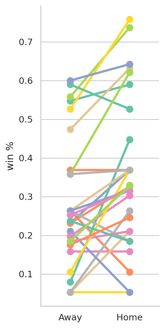
The overall picture shows most teams have a clear advantage at home:

g = sns.FacetGrid(results.reset_index(), hue="team", palette="Set2", height=6, aspect=0.5)
g.map(sns.pointplot, "is_home", "win_pct", order=["Away", "Home"])
g.set_axis_labels("", "win %");

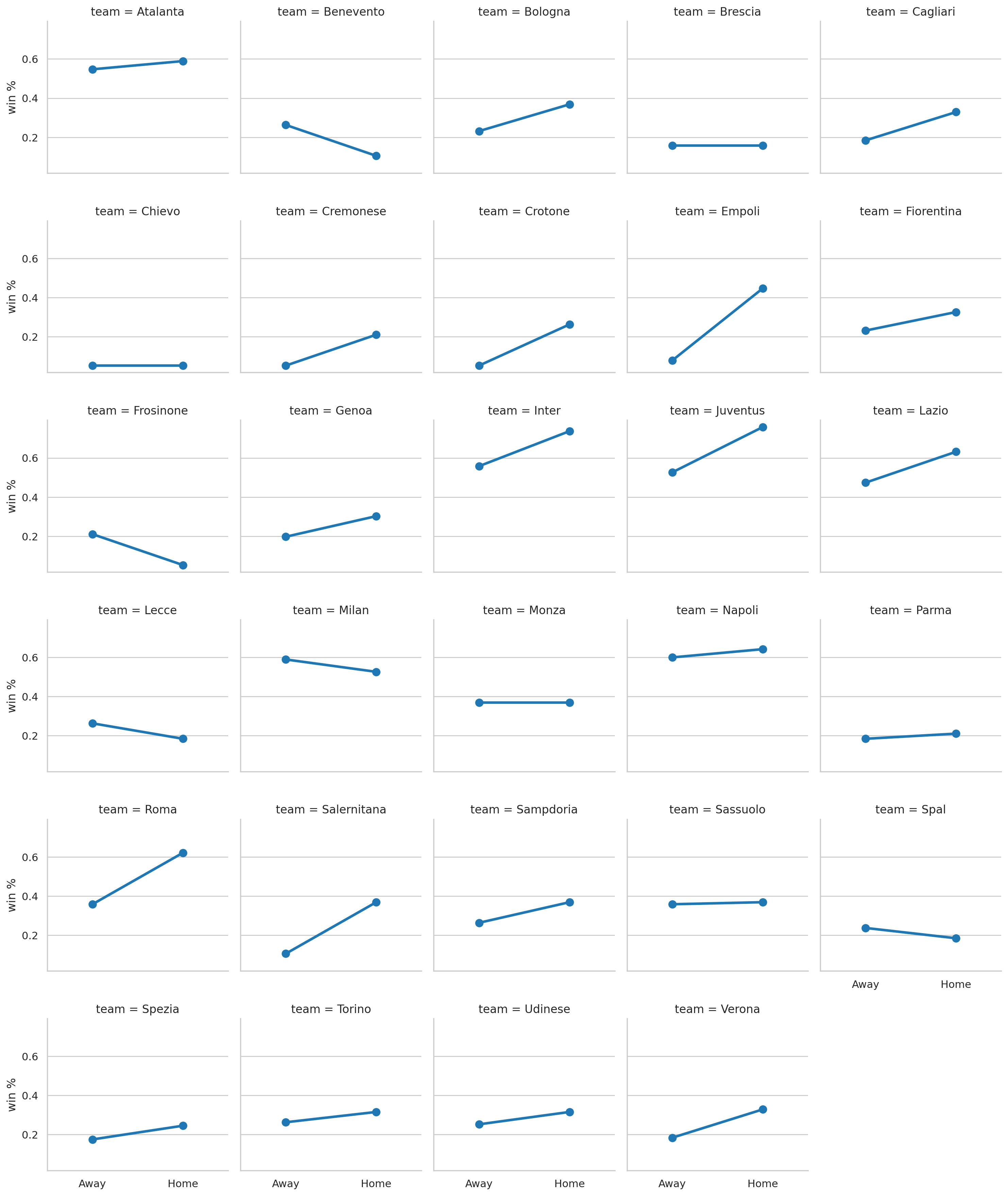
But there are a few exceptions.

g = sns.FacetGrid(results.reset_index(), col="team", col_wrap=5)
g.map(sns.pointplot, "is_home", "win_pct", order=["Away", "Home"])
g.set_axis_labels("", "win %");